自适应Filon积分法
在 固定间隔的Filon积分法 部分简单介绍了Filon积分的过程与核心原理,即 分段计算积分的解析解,而以下介绍的 自适应Filon积分法(SAFIM) ,便是 动态分段,在核函数变化剧烈的部分多采样,在核函数变化平缓的部分少采样。具体原理详见 (Chen and Zhang, 2001) (张海明, 2021) 。
参数介绍
通过以下可选参数,可使用自适应Filon积分。
详见 greenfn 和 static_greenfn 模块的 -L 选项。
compute_grn() 函数和 compute_static_grn() 函数支持以下可选参数来使用自适应Filon积分,具体说明详见API。
Length:float定义离散波数积分的积分间隔 (见 控制波数积分 部分, 固定间隔的Filon积分法 部分)safilonTol:float定义自适应采样精度,见 (Chen and Zhang, 2001) (张海明, 2021),通常1e-2即可。filonCut:float定义了两个积分的分割点, \(k^*=\)<filonCut>\(/r_{\text{max}}\) (见 固定间隔的Filon积分法 部分)
示例程序
使用 -S 导出核函数文件,
#!/bin/bash
rm -rf GRN*

# method 1: DWM
# 使用-H来节省一些时间,只输出单个频率以作示例
grt greenfn -Mmilrow -OGRN1 -N2000/1 -D5/0 -R2500 -L20 -H0.25/0.25  -S

# method 2: SAFIM
# 使用-La指定相关参数
grt greenfn -Mmilrow -OGRN2 -N2000/1 -D5/0 -R2500 -La20/1e-2/10 -S500
import numpy as np
import pygrt

modarr = np.loadtxt("milrow")

pymod = pygrt.PyModel1D(modarr, 5, 0)

st_grn = pymod.compute_grn(
    distarr=[2500],
    nt=2000,
    dt=1,
    Length=20,
    safilonTol=1e-2,  # 自适应采样精度
    filonCut=10,
    delayT0=100,
)[0]
使用以下Python脚本绘制核函数采样点,
import numpy as np
import matplotlib.pyplot as plt
import pygrt

statsdata1 = pygrt.utils.read_statsfile("GRN1_grtstats/milrow_5_0/K_0500_2.50000e-01")
statsdata2 = pygrt.utils.read_statsfile("GRN2_grtstats/milrow_5_0/K_0500_2.50000e-01")
srctype = 'DD_q'

fig, (ax1, ax2) = plt.subplots(2, 1, figsize=(10, 6), sharex=True)
xlim = [0, 0.65]

karr = statsdata1['k']
_filt = np.logical_and(karr <= xlim[1], karr >= xlim[0])
karr = karr[_filt]
Farr = statsdata1[srctype][_filt]
ax1.vlines(karr, -1, 1, lw=0.1)
ax1.plot(karr, np.real(Farr)/np.max(np.real(Farr)), 'o-', ms=0.5, mec='r', mfc='r', c='k', lw=0.5)
ax1.grid()
ax1.set_xlim(xlim)
ax1.set_title(f"Fixed Interval (npts={len(karr)})")

karr = statsdata2['k']
_filt = np.logical_and(karr <= xlim[1], karr >= xlim[0])
karr = karr[_filt]
Farr = statsdata2[srctype][_filt]
ax2.vlines(karr, -1, 1, lw=0.1)
ax2.plot(karr, np.real(Farr)/np.max(np.real(Farr)), 'o-', ms=0.5, mec='r', mfc='r', c='k', lw=0.5)
ax2.grid()
ax2.set_xlim(xlim)
ax2.set_title(f"Self-Adaptive Interval (npts={len(karr)})")

fig.tight_layout()
fig.savefig("safim.png", dpi=300, bbox_inches='tight')
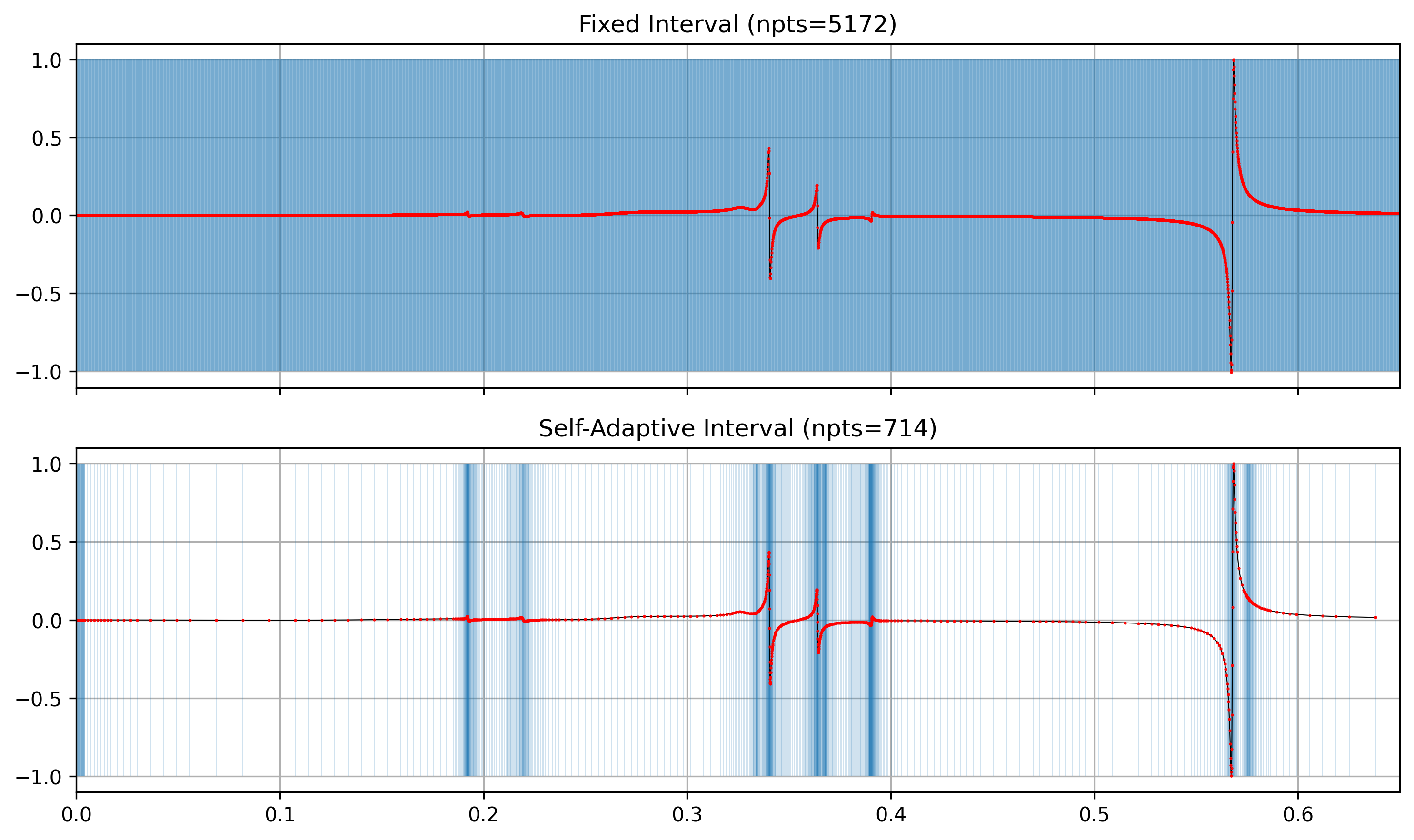
从对比图可以清晰地看出,自适应采样用更少的点数勾勒核函数的主要特征,这显著提高了计算效率。尽管自适应过程增加了额外的计算量,在小震中距范围内计算优势不明显, 但随着震中距的增加,自适应Filon积分的优势将愈发显著。
备注
在程序中,自适应Filon积分不计算近场项,即 计算动态格林函数 中介绍的 \(p=1\) 对应的积分项。